Statistics
Probility and Ramdom Variables
Probability and Simulation
Permutation & Combination
Addition and Multiplication Principle
Permutation
a permutation is the arrangement of objects taken from a ser
The ordir of the objects is important
if there are n distincts objects. we have n! ways of arranging all the objects in a row
if we choose r objects from n distinct objects, wer have nPr ways to arranging the r objects
if some of the objects are identical, the no. of permutations will be less
if there are n objects in total with p identical objects, we have n!/p! ways of arranging all the objects in a row
Conbination
order is not important
there are c ways of selecting r objects
nCr
Circular permutation
Subtopic
each object has two "neighbors" when arranged in a circle
we have (n-1)! wys to arrange n distinct objects in a circle
Simulation
The Idea of Probability
chance behavior is unpredicatable in the short run but has a regular and predictable pattern in the long run
random
individual outcomes are uncertain
a regular distribution of outcomes in a large no. of repetitions
probability of any outcome of a random phenomenon is the proportion of times the outcome would occur in a very large series of reptitions
Probability Models
Sample space
S
the set of all possible outcomes
event
any outcome or a set of outcomes of a random phenomenon
probility modal
a mathematical description of a random phenomenon consisting of two parts
a sample space S
a way of assigning probabilities to event
Probility of an Event with Equal Likely Outcomes
Subtopic
P(A) = n(A)/s(A)
Important Probability Results
0≤P(A)≤1
P(A) =1, event A will certainly occur
P(A)= 0, event A will never occur
P(S) = 1
complement rule
Probability("not" an event) = 1 - Probability(event)


two events A and B are disjoint
mutually exclusive
indenpendent event
chance of one event happen or does not happen doesn't change the probability that the other event occurs
P(A and B) = P(A) * P(B)
General Probability Rules
Conditional probability

A given B
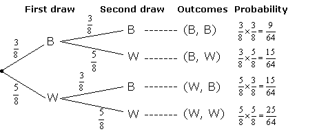
Probability Tree
Random variables
random varible X
A numerical value assigned to an outcome of a random phenomenon.
Discrete and Continuous Random Variables
discrete random variable
random variable with a countable number of outcomes
Probability distribution
a list of the possible values of the DRV together with their respective probabilities
continuous random variable
random variable that assumes values associated with one or more intervals on the number line
Means and Variances of Random Variables

mean

variances

standard deviation
Probility distribution
p(xi) = P(X=xi)
Condition


Probability Density Function

The Binomial and Geometric Distributions
The Binomial Distributions
Subtopic
Bernoulli distribution
Two possible outcomes: "success" or "failure"
p=P(success)
q=P(failure)=1-p
p+q=1
Binomail Distribution
Two outcomes
The experiment is repeated a number of times independently
Conditions
only 2 outcomes in each trial
a fixed number n of trials
trials are independent
probility of success for each trial is the same
Binomial Formula
X be the number of success after n trials
X is binomially distributed with parameters n and p
X~B(n,p)
Binomial distribution is very important in statistics when we wish to make inferences about the proportion p of "success" in a popultaion
Binomial Probability

Probability distribution function
pdf assins a probability to each value of X
Cumulative distribution function
cdf of X calculates the sum of probabilities for 0, 1, 2......, up to the value X
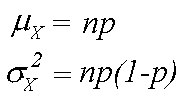
Binomial Mean and Standard Deviation
Normal Approximation to Bionomial Distribution
The formula for binomial probabilities becomes awkward as the no. of trials n increase
When n is large, the distribution of X is approximately Normal
N(np, √np(1-p)
The accuracy of the Normal approximation improves as the sample size n increases
The Geometric Distributions
Geometric Distribution
In a geometric random variable. X counts the number of trals until an event of interest happens
Conditions
Each observation falls into one of just two categories, "success" or "failure"
The observations are all independent
The probability of a success, p is the same for each observation
The variable of interest, X, is the number of trials required to obtain the first success
Calculating Geometric Probabilities
P(X=n) = (1-p)^(n-1)p
Geometric Mean and Standard Deviation
Mean = 1/p
Varience = std^2 = (1-P)/p^2
Sampling Distributions
Sampling Distributions
Parameter & Statistic
A parameter is a number that describes the population
A statistic is a number that can e computed from the sample data without making use of any unknown parameters
Statistics comes from samples while parameters come from populations
Sampling Variability
Different samples will give different values of sample mean and proportion
The value of a statistic varies in repeated random sampling
Sampling Distribution
the distribution of values taken by the statistic in all possible samples of the same size from the same population
Bias and Variability
To estimate a parameter is unbiased
The mean of its sampling distribution is equal to the true value of parameter being estimated
The statistic is called an unbiased estimate of the parameter
Variability
described by the spread of sampling distribution
determined by the sampling design and size of the sample
larger samples give smaller spread
Sample Proportions
The mean of sampling distribution of p is given by p
The standard deviation of the sampling disribution of p is given by √(p(1-p)/n)
Only used when the population is at least 10 times as large as the sample
a Normal approximation
np≥10
n(1-p)≥10
Sample Means
mean of sampling distribution = µ
standard deviation of sampling distribution = std/n
Central Limit Theorem
for large sample size n, the sampling distribution os x is approximately Normal for any population with finite std
the mean and standard deviation of the sampling distribution is given by µ and std/√n
Inference
Estimating with confidence
Confidence Interval
Introduction
Statistical inference
Provides methods fro drawing conclusions about a population from sample data
Estimation
Porcess of determining the value of a population parameter from information provided by a sample statistic
point estimate
a single value that has been calculated to estimate the unknwn parameter
Confidence interval
a range of plausible values that is likely to contain the unknown population parameter
range of values
Subtopic
generated using a set of sample data
center
sample statistics
Confidence Interval and Confidence Level
for a parameter
calculated from the sample data: statistic ± margin of error
gives the probability that the interval will capture the true parameter value in repeated samples
Margin of error

The range of values to the left and right of the point estimate in which the parameter likely lies
Standard error
the standard error of a reported proportion or percentage p measures its accuracy
the estimated standard deviation of that percentage
std/√n
z*std/√n
Confidence interval for a Population Mean
Conditions
sample taken from SRS
Normality: n is at least 30
Independence : population size is at least 10 tmes as large as the sample size
General Procedure for Inference with confidence Interval
Step 1 : state the parameter of interest
Step 2: Name the inference prodedure and check conditions
Step 3: calculate the confidence interval
Step 4: Interpret results in the context of the problem
How Confidence Interval Bheave and Determining Sample Size
smaller margin of error
The confidence level C decreases
the population standard deviation decrease
the sample size increase
Sample size

*E stand for margin of error
Extimating a Population Mean
Std of population unknown
Conditions:
Samples takne from SRS
Population have a normal distribution
Individual observations are dndependent
Standard error of sample mean

*s stand for sample std
The t Distribution
Not normal, it is a t distribution
degree of freedom
df = n-1
because we are using the sample standard deviation s in our calulation
write the t distribution with k degrees of freedom as t(k)
Density curves
similar in shape to the standard Normal curve
The spread of the t distribution is a bit greater than that of the standard Normal distribution
as k increase. the denstiy curve approaches the N(0,1)curve ever more closely

density curve
The One-Sample t confidence Intervals
unknown mean µ
a level C confidence interval for µ is: x ± t*s/√n
t* is the critical value for the t(n-1)
The interval is exactly correct when the population distribution is Normal
The interval approximately correct fro large n in other cases
Paried t Procedures
compare the responses to the two treatments on the same sjubects, applys one sample t procedure
matched pairs design
before-and-after measurement
The parameter µ is a paired t procedure is
the mean difference in the responses to the two treatments within matched pairs of subjects in the entire population
the mean difference in response to the two treatments fro individuals in the population
the mean difference between before-and-after measurements for all individuals in the population
Robustness of t Procedures
robust against non-Normality of the population
not robuts against outliers
Using the t procedures
more important than the assumption that the population distribution is Normal
Sample size less than 15, data close to normal
large samples
Estimating a Population Proportion
Conditions for Inference about a proportion

replace the standard deviation by the SE of p
level C confidence for population proportion: p±z*√(p(1-p)/n)
Conditions:
The datas are taken from SRS
Normality
np≥10
n(1-p)≥10
Individual observations are dndependent
Choosing the sample size
m = z*√(p(1-p)/n)
n=(z*/m)^2 p(1-p)
Testing a Claim
The basics
using a confidence interval to estimate the population parameter
using a statistical test to asses the evidence provided by data about some claim concerning a populatin
Basic ideas
An outcome that would arely happen if a claim were true is good evidence that the claim is not true
How rare is rare
Stating Hypohteses
null hypotheses
the statement being tested in a significance test
H0 : μ1 = μ2
alternative hypotheses
the claim about the population that we are trying to find evidence for
H0 : μ1≠μ2
P-value
The probability of a result at least as far out as the result we actually got
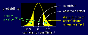
Significant test
Signficance tests are performed to determine whether the ovserved of a sample statistic differs significant from the hypothesized value of a population parameter
porcedure
Step1: Hypothesis
Identity the population of interest and the parameter
State hypotheses
Step 2: Conditions: Choose the appropriate inference procedure
z-Test for population mean
population std known
z = (x-µ)/(std/√(n))
t-Test for population mean
population std unknown
t = (x-µ)/(s/√(n))
Sample from SRS
Samples indenpendent from each other
Sample follow Noraml distribution
Step3: Calculations
Calculate the test statistic
Find the P-value
by GC
value used
µ>µo, p
µ<µo, p
µ≠µo, 2p
Step 4: Interpretation
Interpret the P-value or make a decision about Ho using statistical significance
Conclusion, connection and context
Test from confidene interval
intimate connection between confidence and significance and significance
if we are 95% confident that the true µ kues in the interval, we are also confident that the values of µ that fall outside ourinterval are incompatible with the data
Confidence intervals and Two-Sided Test
a two-sided significance test rejects a hypothesis exactly when the value µo falls outside a level 1- alpha confidence interval for µ
The link between two-sided significance tests and confidence interval is called duality
in two-sided hypothesis test, a significance test and a confidence interval will yield the same conclusion
cannout use a confidence interval in place of a significance test for one-sided tests
Use and Abuse of Tests
valued because an effect that is ulikely to occur simply by chance
choosing a Level of significance
How plausible is Ho
What are the consequedces of rejecting Ho
no sharp border between statistically significan and tattistically insignificant
increasing strong evidence as the P-value decrease
Statistical Significance and Practical Importance
very small effects can be highly significan
A statistically significant effect need not be parctically important
Statistical inference is not valid for all sets of data
Beware of multile analyses
Type I and Type II error
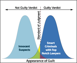
If we reject Ho when Ho is actually true, we have a committed type I error
The significance level of any fixed level test is the probability of type I error
If we fail to reject Ho when Ho is false, we have committed a type II error
power test
when a particular alternative value of parameter is true is called the power of the test againgst that alternative
The power of a test against any alternative is 1 minus the probability of a type II error for that alternative
1-ß
Increase the power of a test
increase alpha
consider a particular alternative that is farther away from µ
Increase the sample size
Decrease std through improving the measurement process and restricting attention to a subpopulation
Significance Tests in Pratice
The one sample t-test
The One-propottion z test
z = P-Po/√(Po(1-Po)/n)
Normality condition
nPo≥10
n(1-Po)≥10
Comparing Two population Parameters
Population std known
Two-Sample z Statistic

Population std unknown
The Two-Sample t procedure
level C confidence interval
two-sample t statistic
Degree of Freedom

software comput
Choose the small one
Two sample tests about a population proportion

Conditions:
SRS
Indenpendence
Normality
Inference for Distribution of Catagorical Variables
The Chi-Sqaures Test fro Goodness of Fit

P-value and significant test
The Chi-Sqaure Distribution
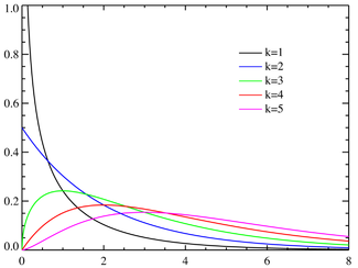
alternative hypothesis: at least one catagory data is different the null hypothesis
df = no. of catagoris-1
The Chi-Square Test for homogeneity of populations
expected count = (row total*column total)/n

Conditions:
SRS
Independence
Normality
Inference for Regression
Analyzing Data
Exploring Data
Displaying Distributions with Graphs
Graphs for Categorical Data
Dotplots

Pie Chart

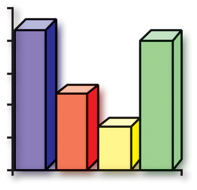
Bar Chart
Graphs for Quantitative Data
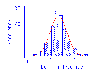
Histrogram
Stemplots

Cumulative Frequency Plots

Time Plots

Subtopic
Describing a Graphical Display
Mode
The mode is one of the major "peaks" in a distribution
Unimodal
distribution with exactly one mode
bimodal
Distribution with 2 mode
Center
The center which roughly separates the values roughly in hafl
Spread
The scope of the valves from the smallest to the largest values
Clusters
The natural subgroups in whch the values fall into
gaps
Holes in which no values fall into
Outliers
Extreme values in the distribution
Due to errors
Requires futher analysis
Due to natural variation in the data
Shape of Graphical Displays

Symmetric
Skewed
Skewed left

Skewed right

Uniformed

Bell-shaped
Describing Distributions with Numbers
Mearuring the Center
Mean
The mean of a series of variables is the arithmetical average of those numbers

Median
The Median is the middle number of a set of a data arranged in nmbrical ascending/descending order
NO. of items is ole
E.g: {3.5,9,15,15},Median=9
NO. of items is ever
E.g:{3,5,9,10,15,15} Median = (9+10)/2
Reisitant Measure
iThe median value is not affected by outlier values. Wd describe the median as a resistant measure.
Measuring Spread
Range:
difference between large and small observation
Percentile
Median, M, the 50 percentile
Q1, the 25 percentile
Q3, the 75 percentile
Interquartile range(IQR)
The difference between the first and third quartile
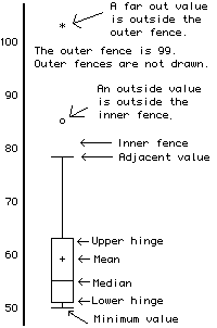
Box Plot
Change Unit of Measures
Comparing Distribution
Describing Location in a Distribution
Mearures of Relative Standing and Density Curves
Position of the Score(How your score compares to other peoples's score)
Z-Score
To measred how many standard deviations is avay from the mean
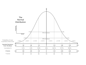

Percentile
The pth percentil of a distribution is defined as the value with p percent of the ovservation less or equal to it
Chebyshey's Inequality
In any distribution, the percentage of observations falling within standard deviation of the mean is at least
Density Curves
A mathematical model for the distribution
Idealized description
Always on or above and horizontal axis
The area underneath is exactly 1
Mean and standard deviation
Mean & Median of Density Curve
Median: "equal-areas point"
Mean:"banlance point"
For different types of curves
Symmeric density curve: Mean = Median
Skewed righta: Mean is on the right side of the median
Skewed lift: Mean is on the left side of the median
Normal Distributions
Normal Distribution
These density curves are symmetric, single-peaked and bell-shaped
Density function
Importance
Often a good descriptor for some distribution of real data
Good approximations to results of many chance outcomes
Many statistical inference procedures based on Normal distribution work well for other roughly symmetrical distributions
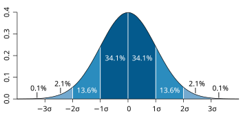
Empirical Rule
Subtopic
About 68% of the values lie within 1 standard deviation of the mean
μ ± σ.
About 95% of the values lie within 2 standard deviations of the mean
μ ± 2σ.
Almost all (99.7%) of the values lie within 3 standard deviations of the mean
μ ± 3σ.
Standard Normal Distribution
A Normal distribution with mean 0 and standard deviation 1
For any Normal distribution we can perform a linear transformation on the variable to obtain an standard Normal distribution
Standard Normal Calculation
Proportion of observations lie in some range of values
Standard normal table
Assesing Normallity
How well the data fit the empirical rule
Histograms
Stem plots
Box plots
A normal probbility plot
Subtopic
If the points on a Normal probility plot lie close to a straight line, the plot indicates the data are Normal
Outliers appear as points that are far away from the overall pattern of the plot
Systematis deviations from a straight line indicate a non-Normal distribution
Examining Relationships
Response Variable and Explanatory Variable
A response variable measures an outcome of a study
An explanatory variable helps explain or influences changes in a response variable
To identify a response and explanatory variable by specifulying values of one variables in order to see how it affects another variable
Explanatory variable does not necessary causes the change in the response variable
Scatterplots and correlation
The relationship between 2 quantitative varibles measured on the same individuals
Plot the explanaory variable as the horizontal axis, and the response variable on the vertical axis
Interpretion a Scatterplot
Look for overall pattern and for striking deviations from that pattern
Outlier: an individual value that falls outside the overall pattern of the relationship
Describe the pattern by the direction, form and strenght of the relationship
Positive & Negative Association
Positive associated
The above-average values and below-average value tend to occur together
Negative associate
above-average values of one tend to accompany below-average values of the other and vice versa
Categorical Variables in Scatterplots
Subtodisplay the different categories
different plot color
different symbol
Correlation
Measrue dircetion and strength of a linear relationship

Between -1 to 1
r near to 0
weak relationship
r near to 1 or -1
strong linear relationship
Does not measure curved relationship between variables
Least Squares Regression Line
Stright line describes how a response varible y changes sa an explanatory varible x changes
predict the value of y
y = a + bx
Least-Squares Regression
Residuals & Residuals Plot
residual
observed y - predicted y
residual plot
how well the regression line fits the data
should show no obvious pattern for liner relationship
Std of residual

Coefficient of Determination
r^2
% of observations lie on least squares regression line

Outliers and Influential Obserbation in Regression
Lurking Variable
not among the explanatory or response variable in a study
Correlation and Regression Wisdom
Correlation: Measuring Linear Association
Correlations Based on Averaged Data
More about Relationships between Two Variable
Transforming to Achieve Linearity
Exponential Growth Model
Dependent variable = log(y) log(y) = b0 + b1x ŷ = 10b0 + b1x
Power Law Model
Dependent variable = log(y) Independent variable = log(x) log(y)= b0 + b1log(x) ŷ = 10b0 + b1log(x)
Relationships between Categorical Variables
Simpon's Paradox

Establishing Causation
Explaing Association
Explaning Causation
Producing Data
Desinging Samples
Observational Study & Experiment
Ovservational study
observe individuals and measure variables of interest
do not attempt to influence the responses
the effect of one variable on another often fail
explanatory variable is confounded with lurking variable
cheaper
experiment
deliberately impose some treatment on individual
observal the responses
allow to pin down the effects of specific variables of interest
Designing Sample
Population and Sample
population
entire group of individuals
census
census attempts to contact every individual in the entire population
advantage
able to find all characteric of the population accurately
disadvantages
expensive
time causing
sample
part of population that we actually examine in order to gather information
sampling
sampling involves studing a part in order to gain information about the whole
advantages
cheaper
less time needed
may miss out centain characteristics of the population
Voluntary response sampling
people who choose themselves by responding to a general appeal
voluntary response bias
people who feel most strongly about an issue are most likely to respond
Convenience Sampling
individuals who are easiest to reach
undercoverage bias
Probability Sample
random sample
each member of the population is equally likely to be included
Simple Random Sampling
A sample of a given size
every possibel sample is equally likely to be chosen
4 steps to choose SRS
1 label
2 table
3 stopping rule
4 identify sample
systematic sample
first member of the sample is chosen according to the some random procedure
the rest are chosen according to some well-defined pattern
Stratified Random Sampling
subgroups of sample, strata appear in approximately the same proportion in the sample as they do in the population
Cluster Sampling
divide population into groups as clusters
randomly select some of the clusters
all the individuals in the chosen clusters are selected to be in the sample
Multi-Stage Sampling Design
Cautions about Sample Surveys
Sampling Bias
Undercoverage
some part of population being sampled is somehow excluded
voluntary response bias
voluntary response bias
self-selected samples
persons who feel most strongly about an issue are most likely to respond
non-response bias
the possible biases of those who choose not to respond
wording bias
wording of the question influences the response in a systematic way
response bias
not give truthful responses to a question
respondent may fail to understand the question
respondent desires to please the interviewer
the ordering of question may influence the response
Desinging Experiments
Design of Experiment
Do something to individuals in order to observe the response
Control
overall effort to mnimize variability in the way experimental unit are obtained and treated
a group reveives the treatment
another group does not reveive any treatment (control group)
compares the responses in reatment group and control group
reduce the problems posed by confounding and lurking variables
placebo
a dummy treatment
Replication
natural variability among the experiment units
reduce the role of variation
increase the sensitivity of the experiment to differences between treatments
Randomizations
divide experimental units into groups by SRS
randomized comparative experiment
ensure that influences other than the treatments operate equally on all groups
completely randomized design
all the experimental units are allocated at random among all treatments
statistically significant
ovserved effect is very large
would rarely occur by chance
Block Design
a group of experimental untis or subjects similar in some way
expected to systematically affect the response to the treatments
random assignment of units to treatments is carried out separately within a block
characteristics
formed based on teh most important unavoidable sources of variability among the experimental units
another form of control, which controls the effects of some outside variables by bring those variables into the experiment to form the blocks
can have any size
chosen based on the likelihood
allows to draw separate conclusions about each block
Matched Pairs Design
an example of block design
compare tow treatments and the subjects are matched in pairs
more similar than unmatched subjects => more effective
Cautions abut Experiment
double-blind experiment
lacking of realism limits ability to apply the conclusions of an experiment to the settings of greater interest
