Kategorien: Alle - variables - linear

von Matthew Jenkins Vor 2 Jahren

94

Chapters 5 and 6

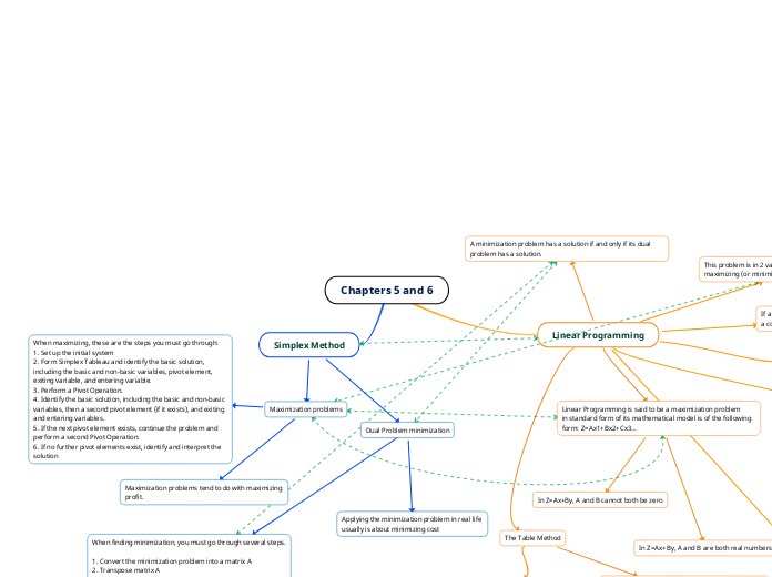
The text provides a detailed guide on solving maximization and minimization problems using the Simplex Method, which is a key technique in linear programming. For maximization problems, the procedure involves setting up the initial system, forming the Simplex Tableau, identifying basic and non-basic variables, and performing pivot operations until no further pivot elements exist.
Chapters 5 and 6

Chapters 5 and 6

Simplex Method

Dual Problem minimization
Applying the minimization problem in real life usually is about minimizing cost
When finding minimization, you must go through several steps. 1. Convert the minimization problem into a matrix A 2. Transpose matrix A 3. Convert the matrix into a dual problem 4. Find the solution to the dual problem 5. The solution to the dual problem is also the solution to the minimization problem
Maximization problems
Maximization problems tend to do with maximizing profit.
When maximizing, these are the steps you must go through: 1. Set up the initial system 2. Form Simplex Tableau and identify the basic solution, including the basic and non-basic variables, pivot element, exiting variable, and entering variable. 3. Perform a Pivot Operation. 4. Identify the basic solution, including the basic and non-basic variables, then a second pivot element (if it exists), and exiting and entering variables. 5. If the next pivot element exists, continue the problem and perform a second Pivot Operation. 6. If no further pivot elements exist, identify and interpret the solution

Linear Programming

Theorem 2
A) If the feasible region for a linear programming problem is bounded, then both the maximum and minimum value of the objective function exist. B) If the feasible region is unbounded, and the coefficients of the objective function are positive, then only the minimum exists. C) If the feasible region is empty (no points satisfy all constraints) then there is no maximum or minimum value.
Step-by-step process to find solution
1. Graph the feasible region. If an optimal solution exists according to Theorem 2, find the coordinates of each corner point. 2. Construct a corner point table and list what the value of the objective function is at each particular corner point. 3. Determine what the optimal solution is from the corner point table. 4. For an applied problem, interpret the optimal solution in terms of the original problem
If a linear programming problem has multiple solutions, it is located along the boudary lines that follow the constant-profit line
If a linear programming problem has a solution, it is located at a corner point
This problem is in 2 variables, x and y, and consists of maximizing (or minimizing) a linear objective function
A minimization problem has a solution if and only if its dual problem has a solution.
The Table Method
To solve a system of inequalities, you must follow these steps: 1. Convert the given i-system to an e-system. To do this you must add slack variables, one per equation. This will lead to 2 equations with 4 unknowns, which means infinite solutions. 2. We can make the system then be able to have a unique solution by assigning two of the variables a value of zero and then solving for the remaining variables (called a basic solution). 3. We select any of the four variables as non-basic. The remaining two become basic. The non-basic variables are always assigned a value of zero. Then we solve the equations for the two basic variables. 4. We repeat step three for every variable combination and summarize the results in a table. 5. When the table is completed you can find the solutions, but take note: A basic solution that is not feasible (does not satisfy all constraints) includes at least one negative value. A basic feasible solution does not include any negative values.
In the table method, you must convert inequalities into equalities (equations). This is called changing an i-system into an e-system.
Linear Programming is said to be a maximization problem in standard form of its mathematical model is of the following form: Z=Ax1+Bx2+Cx3...
In Z=Ax+By, A and B cannot both be zero
In Z=Ax+By, A and B are both real numbers